So I fancied coming back to do writeups after a 4-year hiatus.
This CTF was apparently very easy to one-shot with GPT Plus, and I’m pretty sure none of the top 10 teams solved a majority of the challenges without LLM assistance.
However, I had quite a few interesting concepts and challenges that I found fun to solve (notably, WITHOUT resorting to LLM chatbots). Let’s go.
Writeups
StrideSafe
Singapore's lamp posts are getting smarter. They don't just light the way -- they watch over the pavements.

Your next-gen chip has been selected for testing. Can your chip distinguish pedestrians from bicycles and PMDs (personal mobility devices)?

Pass the test, and your chip will earn deployment on Singapore's smart lamp posts. Fail, and hazards roam free on pedestrian walkways.
Reconnaissance
We are given a zip file containing a 1k 64x64 RGB images. Conspicuously missing are any image labels, leading me to think that:
- This is an unsupervised learning challenge
- The challenge wants us to run inference.
While I can tell you right now that method 2 gave us the flag,
but since this was a LLM-less attempt… let’s just say I wasted a lot of time on method 1. So I’m going to waste YOUR time too >:D
Trying Unsupervised Learning

As mentioned above, there were no image labels. So my first instinct was to perform a quick PCA + K-Means clustering to see if the images could be grouped into 2 distinct clusters (people vs bicycles/PMDs).
# This was done on a Jupyter notebook, so the code snippets are kind of scattered. Sorry!
import glob
from PIL import Image
from matplotlib import pyplot as plt
import numpy as np

# Retrieve all the images and put them into shapes.
image_files = glob.glob("data/*.jpg")
# for img_path in image_files:
#     img = Image.open(img_path)
#     img = img.convert("RGB")

dummy_path = next(iter(image_files), None)
dummy_image = np.array(Image.open(dummy_path)) if dummy_path else None
print(dummy_image.shape)
plt.imshow(dummy_image)

### New cell
import polars as pl
import einops

image_data = []

for img_path in image_files:
    img = Image.open(img_path)
    img_array = np.array(img)
    img_array = einops.rearrange(img_array, "h w c -> (h w c)")
    image_data.append(img_array)

df = pl.from_numpy(np.array(image_data))
print(df.head())

file_names = [img_path.split("/")[-1] for img_path in image_files]
df = df.with_columns(pl.Series("file_name", file_names))
df.write_csv("images.csv")

### New cell
from sklearn.decomposition import PCA
from sklearn.neighbors import NearestNeighbors
from sklearn.manifold import TSNE
from sklearn.cluster import KMeans, DBSCAN
from sklearn.preprocessing import StandardScaler

# Load the CSV file
df = pl.read_csv("images.csv")
X = df.drop("file_name").to_numpy()

# Scale and do dim reduction.
scaler = StandardScaler()
scaled_data = scaler.fit_transform(X)

pca = PCA(n_components=100)
pca_result = pca.fit_transform(scaled_data)
print(f"PCA reduced data shape: {pca_result.shape}")
# print(f"Good threshold for number of components: {np.sum(pca.explained_variance_ratio_ >)}")
print(f"Explained variance ratios: {pca.explained_variance_ratio_}")
thresh = np.sum(pca.explained_variance_ratio_ > 0.01)
print(f"Good threshold for number of components: {thresh}")
print(f"Total explained variance for {thresh} components: {np.sum(pca.explained_variance_ratio_[:thresh])}")

# (1089, 12288)
# PCA reduced data shape: (1089, 100)
# Explained variance ratios: <omitted for sanity>
# Good threshold for number of components: 12
# Total explained variance for 12 components: 0.7005721540268107

### New cell
# Use K-Means clustering
kmeans = KMeans(n_clusters=2, random_state=42, max_iter = 1000)
labels = kmeans.fit_transform(pca_result)

print(f"K-Means labels shape: {labels.shape}")
plt.scatter(labels[:, 0], labels[:, 1], c=kmeans.labels_, cmap='viridis')
plt.title("K-Means Clustering of Image Data")
plt.xlabel("K-Means Component 1")
plt.ylabel("K-Means Component 2")
plt.show()
df_labels = pl.DataFrame(kmeans.labels_, schema=["label"])
pl.concat([df_labels, df["file_name"].to_frame()], how = "horizontal").write_csv("results.csv")
yields a relatively clean clustering of the images into 2 groups:
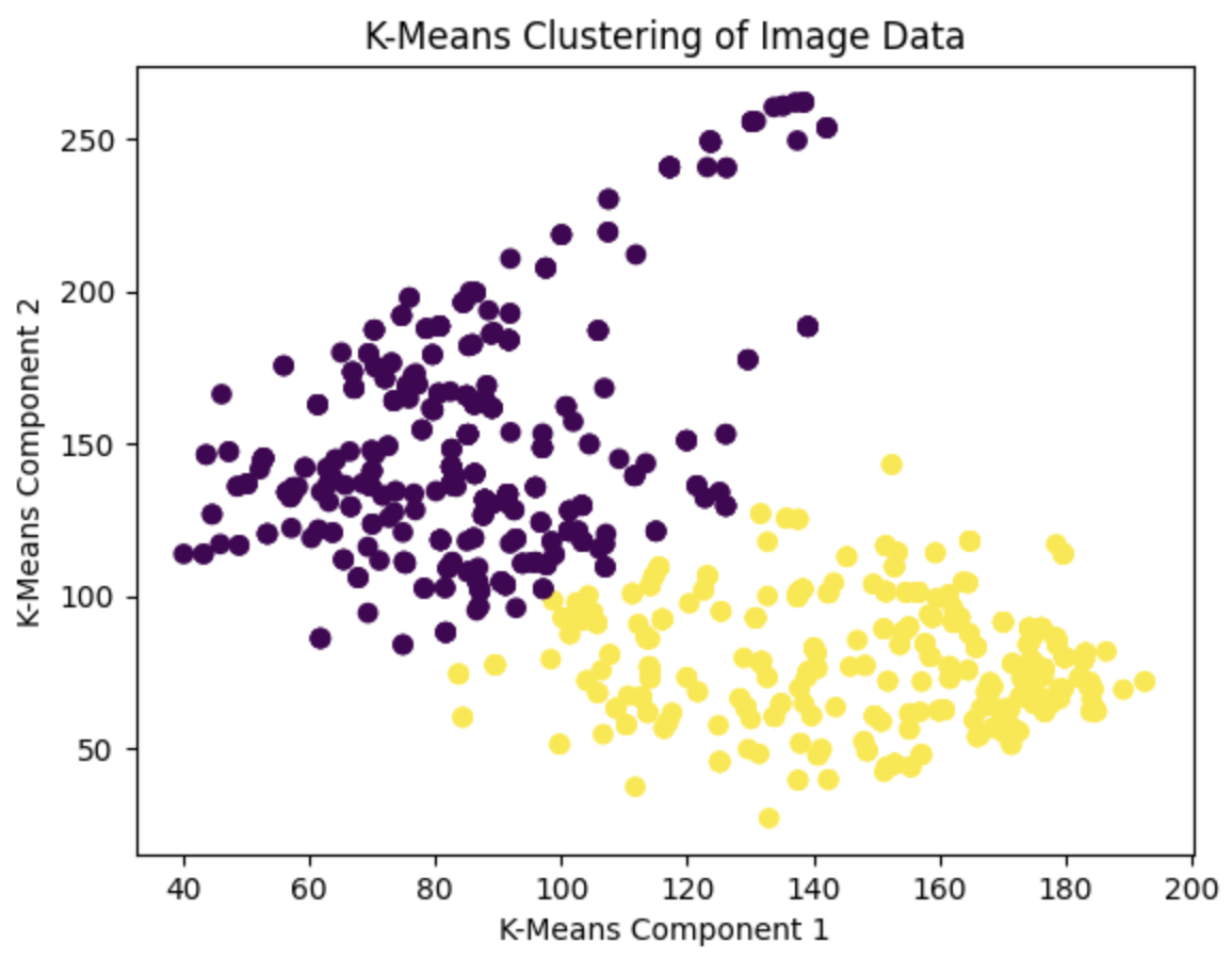
The classification, however, was a lot less clean…
results = pl.read_csv("results.csv").sort(by = "file_name")["label"].to_list()

results_arr = np.array(results)
size = int(np.sqrt(len(results_arr)))

plt.figure(figsize=(3,3))
plt.imshow(1 - results_arr.reshape((size, size)), cmap="gray")
plt.axis('off')
plt.show()

At this point in the contest, you could already sort of make out that the classification results yielded some kind of QR code. But as you can see… it looks nothing like a QR code.
I tried a few things to clean it up, such as:
- Using DBSCAN instead of K-Means
- Using t-SNE instead of PCA
- Tweaking the number of PCA components
- Tweaking the K-Means parameters
But all of these didn’t work.
Trying Inference
So my mind turned instead to the new and fashionable way of doing things: Inference with pre-trained models.
For the record I think that using pre-trained models is quite the cop-out, but cop-outs are encouraged in CTFs since they allow you to get stuff done with less effort…
First model I thought of was OpenAI’s CLIP model, since it is designed to match images to text.
import numpy as np
import polars as pl
import einops
import matplotlib.pyplot as plt
from PIL import Image
import torch
from torch.nn.functional import softmax
import clip
from pathlib import Path
from tqdm import tqdm

CSV_PATH = 'images.csv'  # Update this path
IMG_SHAPE = (64, 64, 3)
MODEL_NAME = 'ViT-B/32'

CATEGORIES = [
    "a photo of a human or person",
    "a photo of a bicycle or PMD",
]

model, preprocess = clip.load(MODEL_NAME, device=device)
model.eval()

df = pl.read_csv(CSV_PATH)
filenames = df["file_name"].to_list()
X = df.drop("file_name").to_numpy()
n_samples = X.shape[0]
images = einops.rearrange(X, "n (h w c) -> n h w c", h=IMG_SHAPE[0], w=IMG_SHAPE[1], c=IMG_SHAPE[2])

if images.max() > 1.0:
    images = images / 255.0

text_inputs = torch.cat([clip.tokenize(c) for c in CATEGORIES]).to(device)

with torch.no_grad():
    text_features = model.encode_text(text_inputs)
    text_features /= text_features.norm(dim=-1, keepdim=True)

predictions, probabilities = [], []

for i in tqdm(range(0, n_samples, BATCH_SIZE), desc="Processing"):
    batch = images[i:i+BATCH_SIZE]

    batch_processed = []
    for img in batch:
        img_uint8 = (img * 255).astype(np.uint8) if img.max() <= 1.0 else img.astype(np.uint8)
        pil_img = Image.fromarray(img_uint8)
        pil_img = pil_img.resize((224, 224), Image.BICUBIC)
        batch_processed.append(preprocess(pil_img))

    image_inputs = torch.stack(batch_processed).to(device)

    with torch.no_grad():
        image_features = model.encode_image(image_inputs)
        image_features /= image_features.norm(dim=-1, keepdim=True)

        similarity = (100.0 * image_features @ text_features.T)
        probs = softmax(similarity, dim=-1)

        batch_predictions = similarity.argmax(dim=-1).cpu().numpy()
        batch_probs = probs.cpu().numpy()

        predictions.extend(batch_predictions)
        probabilities.extend(batch_probs)

predictions = np.array(predictions)
probabilities = np.array(probabilities)

# 0 = human/person, others (i.e. 1) = bicycle/PMD
binary_labels = np.where(predictions == 0, 0, 1)

predicted_confidences = np.array([probabilities[i, pred] for i, pred in enumerate(predictions)])

results_df = pl.DataFrame({
    'file_name': filenames,
    'label': binary_labels,  # 0 = person, 1 = other (bicycle/PMD)
    'confidence': predicted_confidences,
    'detailed_prediction': [CATEGORIES[p] for p in predictions]
})

results_df.write_csv('results.csv')
and with some prompt-engineering, it… kind of worked!

flag: AI2025{5tr1d3s4f3_15_l1t}
Challenge Review
Was a bit annoying, but overall a good beginner challenge. (The writeup elides the fact that prompt engineering took about 30 minutes.)
Limit Theory
Mr Hojiak has inherited a kaya making machine that his late grandmother invented. This is an advanced machine that can take in the key ingredients of coconut milk, eggs, sugar and pandan leaves and churn out perfect jars of kaya. Unfortunately, original recipe is lost but luckily taste-testing module is still functioning so it may be possible to recreate the taste of the original recipe.

The machine has three modes experiment, order and taste-test. The experimental mode allows you to put in a small number of ingredients and it will tell you if the mixture added is acceptable. In order to make great jars of kaya, you have to maximise the pandan leaves with a given set of sugar, coconut milk, and eggs to give the best flavor. However, using too many pandan leaves overwhelms the kaya, making it unpalatable.

Production mode with order and taste-test to check the batch quality will use greater quantities, but because of yield loss, the machine will only be able to tell you the amounts of sugar, coconut milk and eggs that will be used before infusing the flavor of pandan leaves. Plan accordingly.

API: https://limittheory.aictf.sg:5000
https://limittheory.aictf.sg
Reconnaissance
We are given a web interface and an API, as well as a CSV file of sample experiments.

Looking at the CSV file, we see that it contains a list of 800 experiments with 4 input parameters (coconut milk, eggs, sugar, pandan leaves) and a ‘PASSED/FAILED’ output.
coconut_milk,eggs,sugar,pandan_leaves,success
9.556428757689250,2.5347171131856200,3.442141285965060,7132.44787222995,PASSED
7.587945476302650,1.5854643368675200,8.458637582367370,32418.319308810100,FAILED
6.387926357773330,9.539969835280000,4.210779940242300,5612.771975694960,PASSED
...<all the other rows omitted for sanity>...
Like the (torturously long) description suggests, we have 3 API endpoints:
/experiment- takes in quantities of ingredients from a restricted domain, and returns whether the mixture is “acceptable” or not./order- issues ingredient quantities for a production run outside the restricted domain of/experiment./taste-test- takes in the results of the production run, and returns whether the mixture is “acceptable” or not.
It wasn’t apparent from the challenge description, but there was also a pretty severe rate limit of ~120 requests every like 10 minutes? Did not appreciate it, but whatever.
This appears to be a rather classical “fit data and generalize well” machine learning problem; problem being that the model is unknown.
Okay, its ML. So can solve?
Given the pitiful number of experiments provided (800), I immediately suspected that the underlying model was something simple, like a Logistic Regression model.
Just to be safe, I obviously made sure to augment the data by querying the /experiment endpoint with random values within the allowed domain, and adding those to the dataset:
# Also Jupyter notebook code snippets. Sorry!

import aiohttp
import asyncio
import random
import polars as pl
import numpy as np
from tqdm import tqdm
API_URL = "https://limittheory.aictf.sg:5000/experiment"
NUM_SAMPLES = 120
OUTPUT_FILE = "additional_data_new.csv"
NPRNG = np.random.default_rng(42)
RANDOM_SAMPLES = np.concatenate((NPRNG.random((NUM_SAMPLES, 3)), NPRNG.triangular(0, 0.1, 1, (NUM_SAMPLES, 1))), axis=1)

# Restricted domain from website is [0, 10] for first three parameters, and [0, 50000] for last parameter.
RANDOM_SAMPLES[:, :3] *= 10  # Scale first three parameters to [0, 10]
RANDOM_SAMPLES[:, 3] *= 50000  # Scale last parameter to [0, 50000]

async def fetch_sample(session, id, semaphore):
    # Get random parameters to increase dataset support
    async with semaphore:
        params = {
            "coconut_milk": RANDOM_SAMPLES[id, 0],
            "eggs": RANDOM_SAMPLES[id, 1],
            "sugar": RANDOM_SAMPLES[id, 2],
            "pandan_leaves": RANDOM_SAMPLES[id, 3]
        }

        async with session.post(API_URL, json=params) as response:
            label = await response.json()
            params.update(label)
            await asyncio.sleep(0.3)  # Rate limit...
            return params

async def fetch_samples(num_samples):
    semaphore = asyncio.Semaphore(1) # Rate limit...
    async with aiohttp.ClientSession() as session:
        tasks = [fetch_sample(session, i, semaphore) for i in range(num_samples)]
        return [await task for task in tqdm(asyncio.as_completed(tasks))]

# New cell
from time import sleep
for i in tqdm(range(20)):
    samples = await fetch_samples(NUM_SAMPLES)
    pl.DataFrame(samples).write_csv(f"additional_data_batch_{i+1}.csv")
However, I was quite rudely surprised by the level of precision required to pass the /taste-test endpoint:
# New cell
# Try to fit a logistic regressor to the data
from sklearn.linear_model import LogisticRegression
from sklearn.ensemble import RandomForestRegressor
from sklearn.model_selection import train_test_split
from sklearn.metrics import accuracy_score, classification_report
from matplotlib import pyplot as plt
df = pl.read_csv("sample_data.csv")
df = df.vstack(pl.read_csv("additional_data.csv").drop("status").rename({"message": "success"}))
df = df.drop_nulls()
EPS = 1e-8
y = df.select('success').to_numpy()
X = df.drop('success').to_numpy()
print(X.shape, y.shape)
print(df["success"].value_counts())
# New cell
from sklearn.preprocessing import StandardScaler
# Prevent outsized scales from messing with the model...
scaler = StandardScaler()
X = scaler.fit_transform(X)
def pf_map(x):
if isinstance(x, int):
return x
elif isinstance(x, str):
return 1 if x == 'PASSED' else 0
raise ValueError(f"Unexpected value: {x}")
y = list(map(pf_map, y.flatten()))
X_tr, X_val, y_tr, y_val = train_test_split(X, y, test_size=0.2, random_state=42)
clf = LogisticRegression(random_state=42).fit(X_tr, y_tr)
print("Score:", clf.score(X_val, y_val))
print(clf)
# New cell
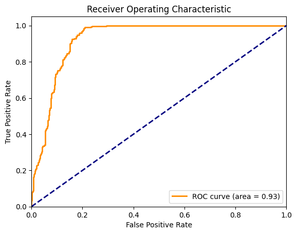
from sklearn.metrics import roc_curve, auc
y_score = clf.decision_function(X_val)
fpr, tpr, _ = roc_curve(y_val, y_score)
roc_auc = auc(fpr, tpr)
plt.figure()
plt.plot(fpr, tpr, color='darkorange', lw=2, label='ROC curve (area = %0.2f)' % roc_auc)
plt.plot([0, 1], [0, 1], color='navy', lw=2, linestyle='--')
plt.xlim([0.0, 1.0])
plt.ylim([0.0, 1.05])
plt.xlabel('False Positive Rate')
plt.ylabel('True Positive Rate')
plt.title('Receiver Operating Characteristic')
plt.legend(loc="lower right")
plt.show()
This is a REALLY GOOD fit. The ROC AUC is 0.93, which is near perfect.
But…
# New cell
import requests
response = requests.get("https://limittheory.aictf.sg:5000/order")
# print("Order response:", response.json())
orders = response.json()['order']
token = response.json()['token']
# Predict the threshold of Pandan leaves for each order
# via binary search on logreg decision function
preds = [0] * len(orders)
for order_name, order in orders.items():
    position = int(order_name.split("-")[-1]) - 1
    low, high = 0, 50000
    for _ in range(30):  # 30 iterations of binary search
        mid = (low + high) / 2
        features = np.array([
            order[0],
            order[1],
            order[2],
            mid
        ]).reshape(1, -1)
        features = scaler.transform(features)
        decision_value = clf.predict(features)[0]
        if decision_value == 0: # i.e. FAIL
            high = mid
        else:
            low = mid
    preds[position] =  (low + high) / 2
# Submit the order
print(preds)
response = requests.post("https://limittheory.aictf.sg:5000/taste-test", json={"token": token, "result": preds})
print("Taste test response:", response.json())
# [15478.281280957162, 7663.008733652532, 10866.082808934152]
# Taste test response: {'RESULT': 'Taste-test failed!'}
# ugh...
So it would seem that we would have to radically revise our approach, perhaps, to model the decision boundary almost perfectly.
This prompted us to believe that some other kind of parameterized linear model was at play here.
Think about it: How else can you get such a clean decision boundary with so few data points?
Linear Modelling
So I decided to try and fit a random assortment of linear models to the data, and see which one fit best.
The key to getting good results with linear models is to do a lot of feature engineering.

Since there are no obvious relationships between the features, I decided to try out a few different transformations (and was prepared to try way more until something stuck):
- Linear (i.e. the original features)
- Ratios (e.g. coconut_milk / eggs)
- Quadratic Forms (e.g. coconut_milk^2, coconut_milk * eggs)
- Logarithmic (e.g. log(coconut_milk))
# Solved again
import polars as pl
import numpy as np
from matplotlib import pyplot as plt
from sklearn.linear_model import LinearRegression

def linear_transform(c, e, s):
    return {
        "c": c,
        "e": e,
        "s": s
    }

def ratio_transform(c, e, s):
    EPS = 1e-8
    return {
        "c/s": c / (s + EPS),
        "e/s": e / (s + EPS),
        "c/e": c / (e + EPS),
    }

def log_transform(c, e, s):
    EPS = 1e-8
    return {
        "log_c": np.log(c + EPS),
        "log_e": np.log(e + EPS),
        "log_s": np.log(s + EPS),
    }
def quadratic_form_transform(c, e, s):
    return {
        "c2": c**2,
        "e2": e**2,
        "s2": s**2,
        "ce": c*e,
        "cs": c*s,
        "es": e*s,
        "c": c,
        "e": e,
        "s": s
    }

df = pl.read_csv("scaling_results.csv")
df = df.drop([
    "base_idx", "scale_factor", "sum"
])

for trf in [linear_transform, ratio_transform, log_transform, quadratic_form_transform]:
    trf_df = pl.DataFrame({
        **trf(
            df["coconut"],
            df["eggs"],
            df["sugar"]
        ),
        "threshold": df["threshold"]
    })
    X = trf_df.drop("threshold")
    y = trf_df.select("threshold")
    print("Transform:", trf.__name__)
    print("X shape:", X.shape, "y shape:", y.shape)
    model = LinearRegression().fit(X, y)
    print("R^2:", model.score(X, y))
    print("MSE:", np.mean((model.predict(X) - y)**2))
    print(f"Names: {model.feature_names_in_}")
    print(f"Coefficients: {model.coef_}, Intercept: {model.intercept_}")
which yielded the following results:
Transform: linear_transform
X shape: (113, 3) y shape: (113, 1)
R^2: 0.9041112446001132
MSE: 1862281.5837982614
Names: ['c' 'e' 's']
Coefficients: [[1008.06767668 320.96307759 1122.20767127]], Intercept: [-5301.56386984]
Transform: ratio_transform
X shape: (113, 3) y shape: (113, 1)
R^2: 0.085363747702359
MSE: 17763399.27893326
Names: ['c/s' 'e/s' 'c/e']
Coefficients: [[-293.16913969 -23.31295561 112.94870038]], Intercept: [4931.46113844]
Transform: log_transform
X shape: (113, 3) y shape: (113, 1)
R^2: 0.7198056157049848
MSE: 5441731.301863531
Names: ['log_c' 'log_e' 'log_s']
Coefficients: [[2935.45798492 1132.50190739 2960.3670994 ]], Intercept: [-3014.31000086]
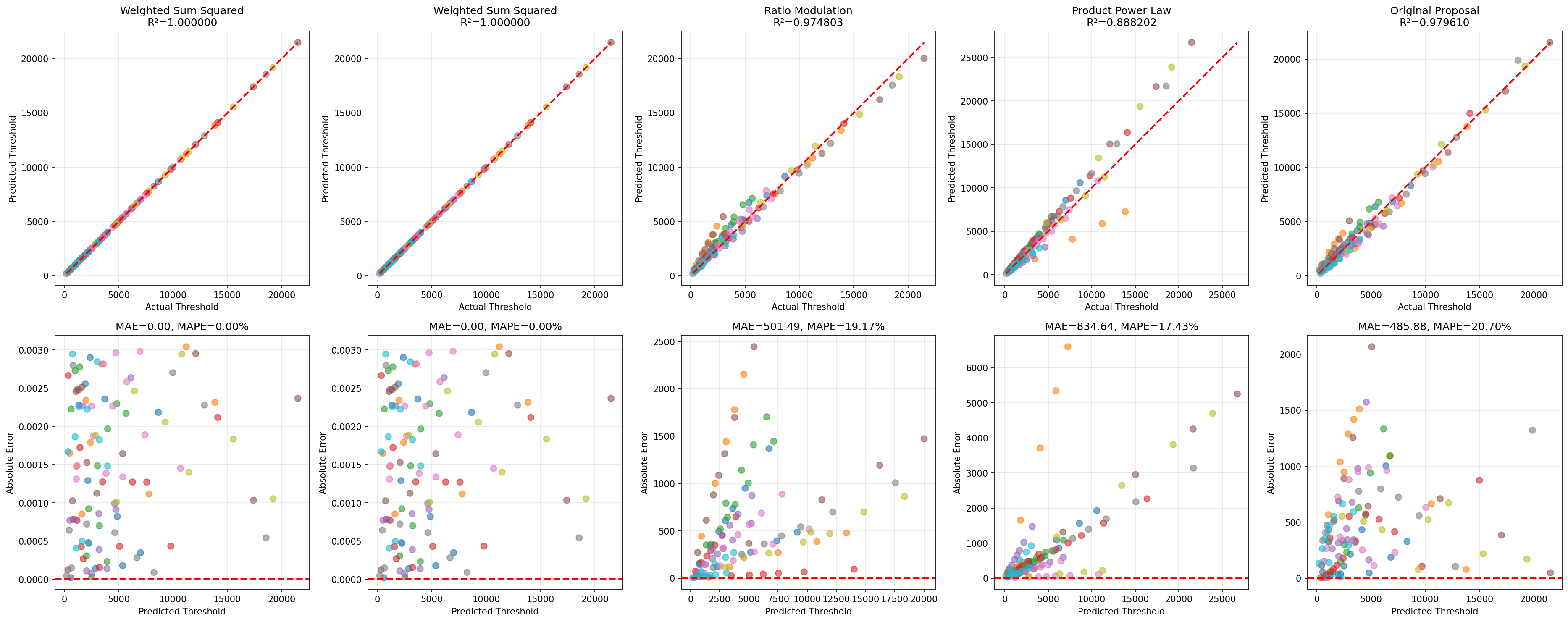
Transform: quadratic_form_transform
X shape: (113, 9) y shape: (113, 1)
R^2: 0.9999999999998537
MSE: 2.841802828936823e-06
Names: ['c2' 'e2' 's2' 'ce' 'cs' 'es' 'c' 'e' 's']
Coefficients: [[-2.19481179e-05 1.80340482e-05 3.24891983e-05 4.99999541e+01
2.00000001e+02 2.00000186e+01 4.72554194e-04 -1.61247451e-05
-3.75376121e-04]], Intercept: [-0.00063777]
Bingo. The quadratic form transformation yielded a near-perfect fit, with an R^2 of 0.9999999999998537.
Let’s try it out:
import requests
best_fn = quadratic_form_transform
trf_df = pl.DataFrame({
    **best_fn(
        df["coconut"],
        df["eggs"],
        df["sugar"]
    ),
    "threshold": df["threshold"]
})
X = trf_df.drop("threshold").to_numpy()
y = trf_df.select("threshold").to_numpy()
model = LinearRegression().fit(X, y)

def predict_pandan_threshold(coconut, eggs, sugar):
    return model.predict(np.array([[
        *best_fn(coconut, eggs, sugar).values()
    ]])).item()

response = requests.get("https://limittheory.aictf.sg:5000/order")
orders = response.json()['order']
token = response.json()['token']

preds = [0] * len(orders)
for order_name, order in orders.items():
    position = int(order_name.split("-")[-1]) - 1
    preds[position] = predict_pandan_threshold(order[0], order[1], order[2])
# Submit the order
print(preds)
response = requests.post("https://limittheory.aictf.sg:5000/taste-test", json={"token": token, "result": preds})
print("Taste test response:", response.json())

# [34289.220314496735, 19659.9614213712, 21017.5142869692]
# Taste test response: {'FLAG': 'AI2025{L1m1t_Th3ory_4_Kaya_T0ast}'}
And just like that, we win!
flag: AI2025{L1m1t_Th3ory_4_Kaya_T0ast}
A Quick Disclaimer
Yes, I made it sound super easy. But in reality this was a 3-hour process of:
- coming up with ideas
- implementing them (with Copilot. I know I said no LLMs, but technically it only provides completions, not solutions)
- testing them
- failing
- repeat
So I got a little tilted when this happened:

(jk, well done Vincent!)
I guess there’s something to be said here about:
- experience and intuition on datasets
- being able to rapidly prototype and test ideas
- luck
- the gulf between challenge setters’ and solvers’ perceptions of difficulty
But they won’t be in this writeup. So there.
Challenge Review
For all the pain I went through only to be outdone by Vincent (& Chad Jippity), I have to say that this was an interesting challenge that presented me a rare opportunity to do Exploratory Data Analysis.
Feature engineering is also rather underrated in favor of architectural improvements and “throwing more compute and data at the problem”, so it was nice to be reminded of its importance.
However, I would have liked if the model was a bit more complex and noisy and the checker a bit less strict, so that more models could have worked. But I don’t know if that would have made it Jippity-able anyways…
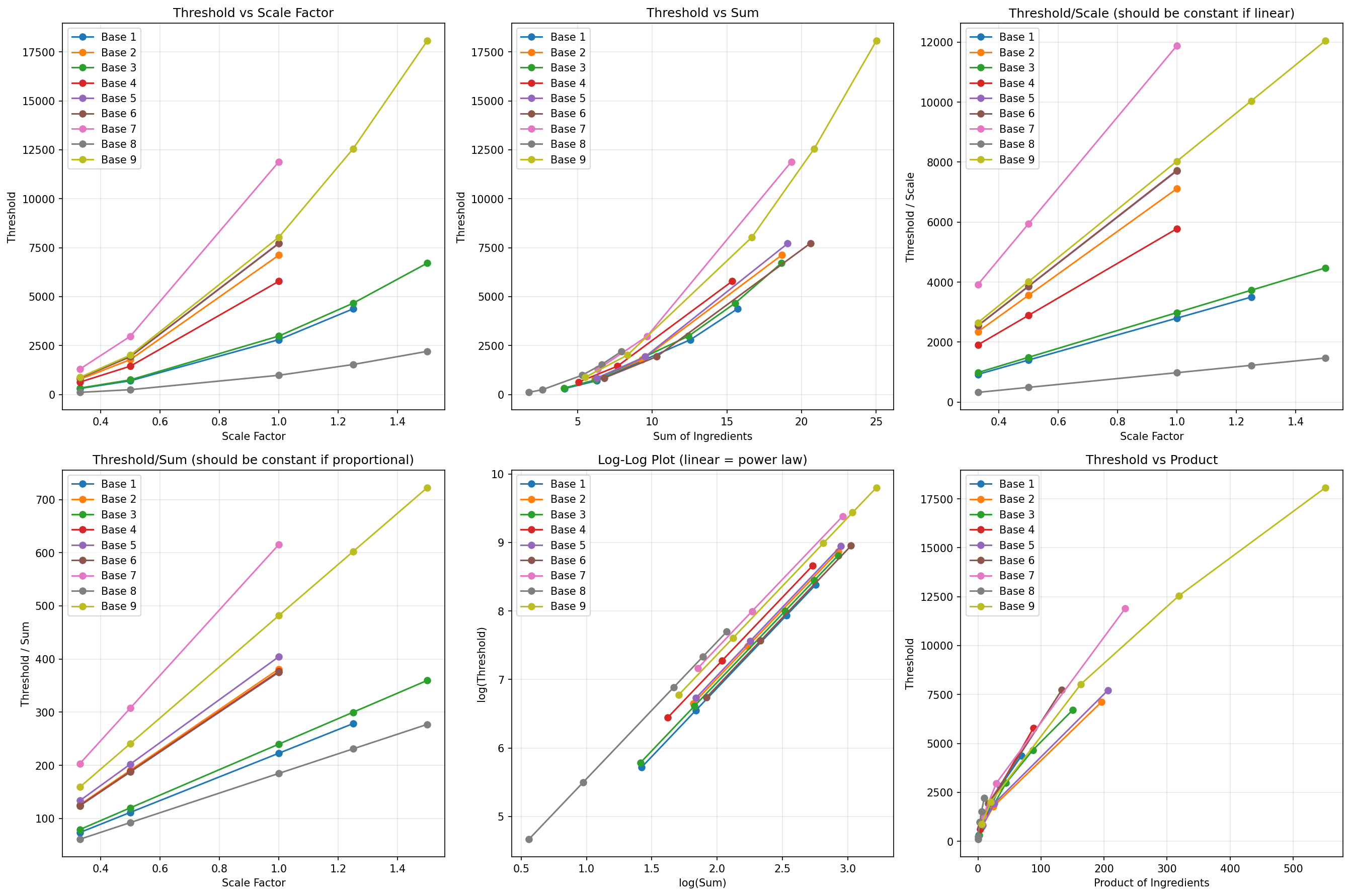
Post-Script: Some Nice Plots
I spent 3 hours querying the /experiment endpoint, getting rate-limited to no tomorrow, WHILE STILL trying to fit various models to the data. So I might as well show you some of the plots that transpired from all that messing around…